消息队列中的排队理论
1,单队列单消费者
MQ中默认一个队列只对应一个消费者,假设单位时间内新来
M/M/1系统1。队列中消息的到达和消费可以建模为生灭过程2,假设有
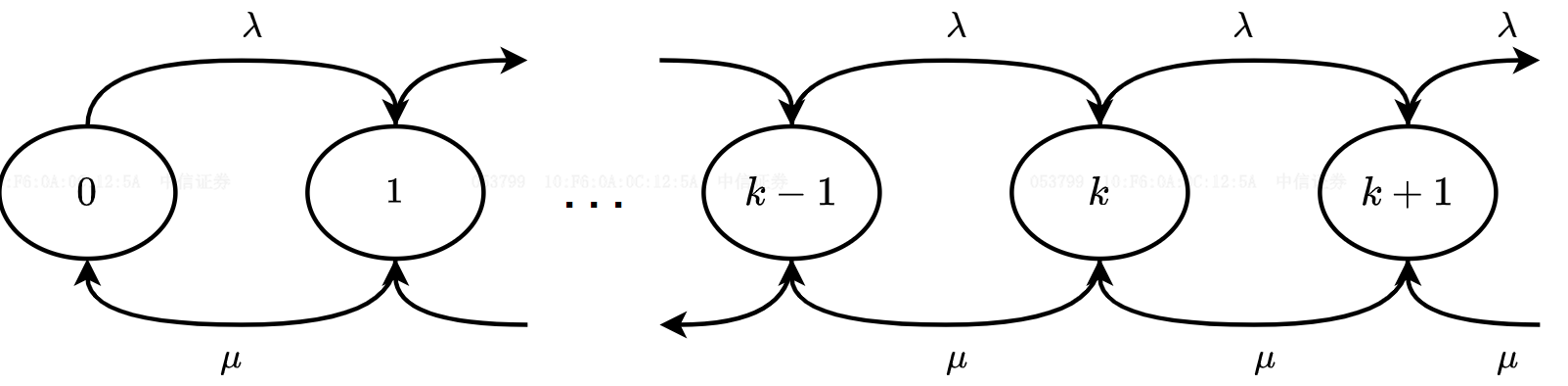
如果队列在状态
对于
对于
结合上述两式可以获得
队列全部状态的概率和为一
系统消息总数均值为处于各个状态的概率和:
等待消息总数均值为系统消息总数均值减去正在处理的消息数:
应用
Little Law3获得消息在系统的平均逗留时间:应用
Little Law获得消息在队列中平均等待时间:
2,单队列多消费者
MQ开启批量消费,一个队列对应
n个消费者,多个消费者共享同一个队列,假设单位时间内新到达M/M/n系统4。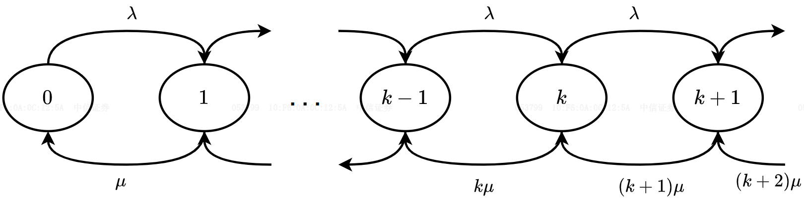
如果队列消息数小于消费者数
如果队列消息数小于消费者
如果队列在状态
对于
对于
对于
综合上式递推得到系统空闲概率
在队列中等待处理的消息总数均值为:
系统平均消息总数均值为处于等待状态的消息总数均值加上正在处理的消息总数均值:
应用
Little Law获得消息在系统的平均逗留时间均值:应用
Little Law获得消息在队列中平均等待均值时间:
3,性能对比
现在假设有5个消费者
n=5,每个消费者单位时间内可以处理一条消息对于n个单队列单消费者构成的系统,定义系统负载
对于包含n个消费者的单队列多消费者系统,定义系统负载
当二者系统负载相同时,将在单位时间内收到相同数量的新消息。下图展示了二者在相同系统负载时队列中等待处理的消息总数均值
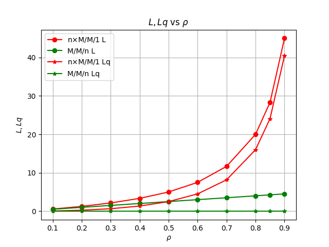
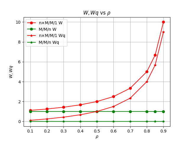
可见当新消息到来速度小于系统消息消费能力
M/M/n系统能立即处理新到来消息,没有消息积压,也没有等待处理耗时。然而单队列单消费者系统相较于单队列多消费者系统,消息积压较为严重,消息等待处理时间更长,在系统负载增大时,劣势更加明显。
4,性能优化
MQ出于消息顺序性消费考虑、以及单个队列读写性能受限的原因,默认限制每个分区只能由一个消费者组中的一个消费者消费。
M/M/1和M/M/n系统性能差距主要来源于:由于队列间独立,并且没有类似Golang中GMP的消息窃取机制(同样出于有序性要求),当一些队列面临高压力出现长队列,而其他队列可能暂时空闲,相应空闲队列对应的消费者空转,导致系统资源利用率低,消息不能及时处理。MQ的解决方式是使用再平衡机制,在消费者与队列之间动态地重新分配队列来实现负载平衡。再平衡机制将在周期性延迟、消费者发生变化,以及订阅topic变化后,被触发执行再平衡。
4.1,RocketMQ 再平衡实现
Rocket MQ中在
RebalanceService#run()中定时(默认20s)触发再平衡流程。1// RebalanceService#run()2public void run() {3long realWaitInterval = waitInterval;4while (!this.isStopped()) {5// 定时休眠后触发再平衡6this.waitForRunning(realWaitInterval);7boolean balanced = this.mqClientFactory.doRebalance();8}9}10}具体通过
RebalanceImpl实施平衡:再平衡过程中,获取当前所有活跃的消费者列表和所有队列的列表,然后根据轮询或者一致性哈希分配等算法将topic下队列分配给所有活跃的消费者。xxxxxxxxxx91// RebalanceImpl#doRebalance()2public boolean doRebalance(final boolean isOrder) {3// 获取当前所有活跃的消费者列表和所有队列的列表4for (final Map.Entry<String, SubscriptionData> entry : subTable.entrySet()) {5final String topic = entry.getKey();6// 执行再平衡7boolean result = this.rebalanceByTopic(topic, isOrder);8}9}xxxxxxxxxx161// RebalanceImpl#rebalanceByTopic2private boolean rebalanceByTopic(final String topic, final boolean isOrder) {3// 获取topic对应的队列和consumer信息4Set<MessageQueue> mqSet = this.topicSubscribeInfoTable.get(topic);5List<String> cidAll = this.mQClientFactory.findConsumerIdList(topic, consumerGroup);6// 选择再平衡策略7AllocateMessageQueueStrategy strategy = this.allocateMessageQueueStrategy;8// 完成再平衡9List<MessageQueue> allocateResult = null;10allocateResult = strategy.allocate(11this.consumerGroup,12this.mQClientFactory.getClientId(),13mqAll,14cidAll);15}16}再平衡策略决定队列和消费者间的对应关系,RocketMQ提供了下列分配策略
AllocateMessageQueueAveragely:默认策略,先计算队列数除以消费者数的余数AllocateMessageQueueAveragelyByCircle:每个消费者依次分配一个队列,循环分配,直至分配完毕全部队列。AllocateMessageQueueConsistentHash:通过一致性hash算法计算队列所属消费者。此策略可以尽量减少 因为队列或者消费者数量发生变化,导致消费者与队列关联关系变化,从而需要重新建立TCP连接的数量。同时再平衡阶段消费者将不能正常消费消息,更少的关系变化,可以更快的完成再平衡过程,减少MQ不可用时间。
4.2,Kafka 再平衡实现
再平衡流程将在消费者组或者topic发生变化后,当前消费者组领导者加入消费组后进行
xxxxxxxxxx131// ConsumerCoordinator#onJoinComplete2protected void onJoinComplete(int generation, String memberId, String assignmentStrategy, ByteBuffer assignmentBuffer) {3// 再平衡策略4ConsumerPartitionAssignor assignor = this.lookupAssignor(assignmentStrategy);5// 待分配分区6SortedSet<TopicPartition> assignedPartitions = new TreeSet(COMPARATOR);7assignedPartitions.addAll(assignment.partitions());8// 执行分配9firstException.compareAndSet((Object)null, this.invokeOnAssignment(assignor, assignment));10this.subscriptions.assignFromSubscribed(assignedPartitions);11firstException.compareAndSet((Object)null, this.invokePartitionsAssigned(addedPartitions));12}13}再平衡策略:Kafka提供了和RocketMQ相似的分配策略
RangeAssignor与RocketMQ的AllocateMessageQueueAveragely策略一致。RoundRobinAssignor与RocketMQ的AllocateMessageQueueAveragelyByCircle策略一致。StickyAssignor:分配尽量均匀,尽量与上一次分配的相同,尽量减少分配关系的变动,从而减少需要重新建立消费者与分区之间TCP连接的数量,缩短再平衡过程耗时,降低MQ不可用时间。。CooperativeStickyAssignor:两阶段再平衡策略,先尝试只移动最少量的分区完成再分配,如果分配后不满足平衡条件,再进行完整的再平衡。
附录
队列长度与逗留时间计算绘制脚本
x
1from scipy.special import factorial2import numpy as np3import matplotlib.pyplot as plt4
5
6# MM1 队列模型7def mm1_queue(lambda_, mu):8 if lambda_ >= mu:9 return "系统不稳定"10 rho = lambda_ / mu11 # 等候+服务人数12 L = rho / (1 - rho)13 # 等候+服务时间14 W = 1 / (mu - lambda_)15 # 等候人数16 Lq = rho**2 / (1 - rho)17 # 等候时间18 Wq = rho / (mu - lambda_)19 return L, W, Lq, Wq20
21# MMn 队列模型22def mmn_queue(lambda_, mu, n):23 # 计算流量强度24 rho = lambda_ / (n * mu)25 if rho >= 1:26 return "系统不稳定,请确保 rho < 1"27
28 # 计算P029 sum_p = sum((lambda_ / mu)**k / factorial(k) for k in range(n))30 p0 = (sum_p + (lambda_ / mu)**n / (factorial(n) * (1 - rho)))**(-1)31 # 计算队列中的平均客户数 Lq32 lq = (rho**n * rho / factorial(n)) * p0 / (1 - rho)**233 # 计算平均等待时间在队列中 Wq34 wq = lq / lambda_35 # 计算系统中的总平均客户数 L36 l = lq + lambda_ / mu37 # 计算系统中的总平均等待时间 W38 w = wq + 1 / mu39
40 return l, w, lq, wq41
42
43
44def plot(x, y, y_label):45 # 绘制图表46 plt.figure()47 # 绘制等待时间48 plt.plot(x, y[0], label="M/M/1", marker='o')49 plt.plot(x, y[1], label="M/M/n", marker='o')50 plt.title(y_label+" vs $\\rho$")51 plt.xlabel("$\\rho$")52 plt.ylabel(y_label)53 plt.legend()54 plt.grid(True)55
56
57# 利用率从0.1到0.958rho_values = [0.1,0.2,0.3,0.4,0.5,0.6,0.7,0.8,0.85,0.9]59mu = 160# 服务台数量61n = 5 62
63# 客户到达率64lambda_ = rho_values*mu 65mm1_array = np.zeros((len(rho_values), 4))66mmn_array = np.zeros((len(rho_values), 4))67
68for i in range(len(rho_values)):69 lam = lambda_[i]70 mm1_array[i] = mm1_queue(lam, mu)71 mmn_array[i] = mmn_queue(n*lam, mu, n)72
73plt.figure()74# 绘制队列长度75plt.plot(rho_values, n*mm1_array[:, 0], label="n$\\times$M/M/1 L", marker='o', color='r')76plt.plot(rho_values, mmn_array[:, 0], label="M/M/n L", marker='o', color='g')77plt.plot(rho_values, n*mm1_array[:, 2],78 label="n$\\times$M/M/1 Lq", marker='*', color='r')79plt.plot(rho_values, mmn_array[:, 2], label="M/M/n Lq", marker='*', color='g')80plt.title("$L,Lq$"+" vs $\\rho$")81plt.xlabel("$\\rho$")82plt.ylabel("$L,Lq$")83plt.legend()84plt.grid(True)85
86plt.figure()87# 绘制等待时间88plt.plot(rho_values, mm1_array[:, 1], label="n$\\times$M/M/1 W", marker='o', color='r')89plt.plot(rho_values, mmn_array[:, 1], label="M/M/n W", marker='o', color='g')90plt.plot(rho_values, mm1_array[:, 3],91 label="n$\\times$M/M/1 Wq", marker='*', color='r')92plt.plot(rho_values, mmn_array[:, 3], label="M/M/n Wq", marker='*', color='g')93plt.title("$W,Wq$"+" vs $\\rho$")94plt.xlabel("$\\rho$")95plt.ylabel("$W,Wq$")96plt.legend()97plt.grid(True)98
99plt.show()100